Unsupervised integration of nasopharyngal carcinoma datasets using EmbedMNN model

In this example, we will use transmorph to integrate nasopharyngal carcinoma (NC) datasets from fourteen patients, gathered in [1]. These datasets contain in total more than 60,000 cells, which are all associated with a cell type annotation among B cell, endothelial, epithelial and macrophage, malignant, NK cell, plasma and T cell. This data bank is challenging for several reasons: large number of batches and cell types, high number of cells, many batches missing some cell types.

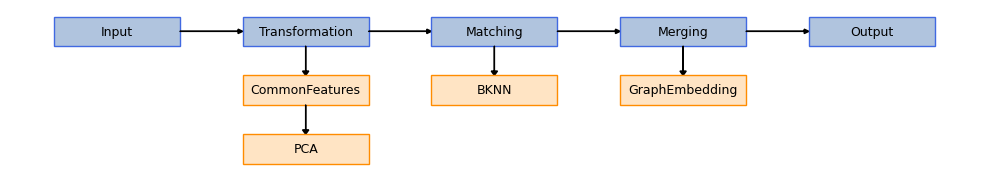
We use one of our built-in models, EmbedMNN, to carry out the integration. It combines a few preprocessing steps (common genes space embedding, normalization and dimensionality reduction) with a mutual nearest neighbors (MNN)-based matching [2] and a low-dimensional space embedding using UMAP [3] or MDE [4]. This low dimensional space can subsequently be used to carry out tasks such as clustering. This is a schematic view of EmbedMNN architecture that can be automatically plotted by transmorph.

from transmorph.models import EmbedMNN
from transmorph.utils.plotting import plot_model

model = EmbedMNN()
plot_model(model)

Loading the data bank

transmorph provides a few data banks for testing purposes, already preprocessed (cell/gene filtering, normalization, log1p…) and annotated. They can be loaded using datasets module. NC databank contains 14 datasets in the AnnData format, each expressed within its 10,000 most variable genes space. Cells are annotated by the .obs key “class”. If the queried databank is missing, it will be automatically downloaded, and saved locally for faster subsequent access.

Typical input data type consists in a dictionary linking a batch name to an AnnData object.

from transmorph.datasets import load_chen_10x

# Format: {patient_label -> AnnData}
chen_10x = load_chen_10x()

databank_api > Loading bank chen_10x.
databank_api > Bank chen_10x successfully loaded.

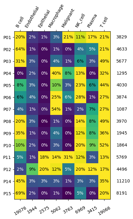
We can first call a transmorph description function to have a closer look at our databank, providing the .obs key containing cell annotations, “class”. We can then observe dataset and annotation distribution across our databank.

# Displaying cell type distribution across batches

from transmorph.utils.plotting import plot_label_distribution_heatmap

plot_label_distribution_heatmap(chen_10x, label="class")

Plotting initial datasets with scatter_plot

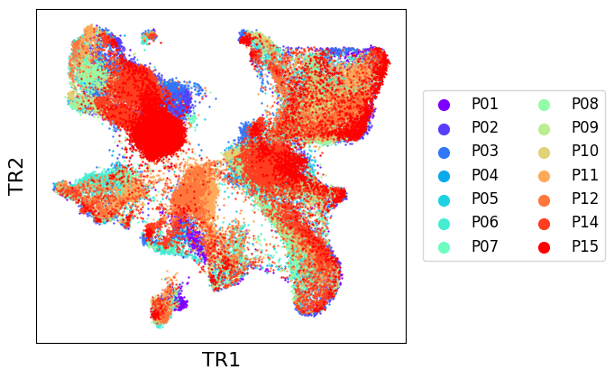
The scatter_plot method can be used to display a low dimensional representation of a set of datasets. It requires first a dimensionality reduction, which can be applied using our framework, we will use the default reducer, UMAP [3]. Computing a UMAP representation can take some time for large datasets, but it can then be cached to avoid recomputing every time.

from transmorph.utils.plotting import scatter_plot, reduce_dimension

reduce_dimension(chen_10x, output_obsm="tr_umap")

scatter_plot(chen_10x, use_rep="tr_umap")
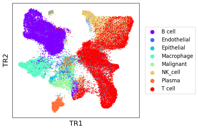
scatter_plot(chen_10x, color_by="class", use_rep="tr_umap")

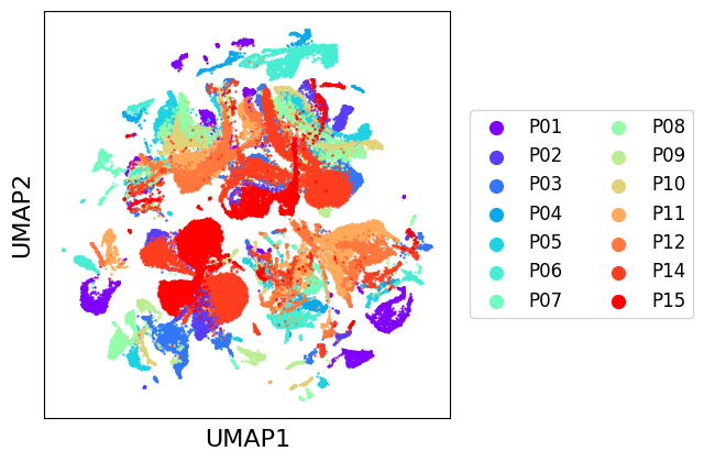
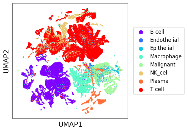
As we can see, there seems to be a general natural clustering of cell types. Though, we observe very important variations between batches, that MNNCorrection will aim to correct. We can assess integration quality using LISI introduced with Harmony [4], which gives an estimation of the number of different labels in the neighborhood of a cell. We use “LISI-batch” with batches as labels to evaluate mixing (higher is better mixed), and “LISI-class” with cell types as labels to evaluate cell types separation (lower is more pure).

from transmorph.stats.lisi import lisi

datasets = list(chen_10x.values())
lisi_batch_bef = lisi(datasets, obsm="tr_umap") # By default, gene representation is used
lisi_class_bef = lisi(datasets, obsm="tr_umap", obs="class")

# Plotting LISI as violin plots

import matplotlib.pyplot as plt
import matplotlib.patches as mpatches
import numpy as np

def add_label(violin, label):
    color = violin["bodies"][0].get_facecolor().flatten()
    labels.append((mpatches.Patch(color=color), label))

positions = np.arange(len(datasets))

labels = []
plt.figure(figsize=(6,4))
add_label(plt.violinplot(lisi_batch_bef, positions=positions - .15), "Batch")
add_label(plt.violinplot(lisi_class_bef, positions=positions + .15), "Class")
plt.xticks(positions, chen_10x.keys(), rotation=90)
plt.xlabel("Batch")
plt.ylabel("LISI")

plt.legend(*zip(*labels), loc=2)
pass

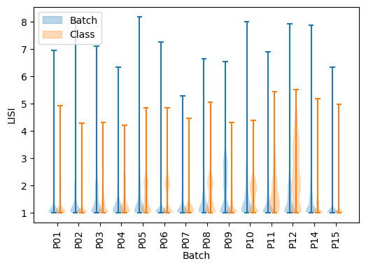
As we can see, except for P10 all batches have only same-batches cells in their neighborhood, and cell type purity is quite decent except for P05, P06, P08, P10 and P12. The goal of integration is to increase LISI-batch while keeping LISI-class as low as possible.

Dataset integration using EmbedMNN

EmbedMNN combines a mutual nearest neighbors step with a graph embedding using UMAP. Parameters can be tuned during model instanciation. Model can then be ran using transform() method, providing a list of AnnData objects and a reference AnnData. The method will add a .obsm[“transmorph”] entry, corresponding to the integrated view computed. We choose not to provide annotations to simulate a completely unsupervised case. This model embeds all datasets in a common genes space, therefore there must exists a nonempty intersection between all .var_names.

model.transform(chen_10x)

EMBED_MNN > Transmorph model is initializing.
EMBED_MNN > Ready to start the integration of 14 datasets, 61870 total samples.
EMBED_MNN > Running layer LAYER_INPUT#0.
EMBED_MNN > Running layer LAYER_TRANSFORMATION#1.
EMBED_MNN > Running layer LAYER_MATCHING#2.
LAYER_MATCHING#2 > Calling matching MATCHING_MNN.
EMBED_MNN > Running layer LAYER_MERGING#3.
LAYER_MERGING#3 > Running merging MERGING_GRAPH_EMBEDDING...
EMBED_MNN > Running layer LAYER_OUTPUT#4.
EMBED_MNN > Terminated. Total embedding shape: (61870, 2)
EMBED_MNN > Results have been written in AnnData.obsm['X_transmorph'].

Integration analysis with LISI

We can then have a look at the final embedding, stored in the .obsm field “transmorph”. It can be passed as input to scatter_plot function.

### Integration analysis with LISI

scatter_plot(chen_10x, use_rep="transmorph", xlabel="TR1", ylabel="TR2")
scatter_plot(chen_10x, use_rep="transmorph", color_by="class", xlabel="TR1", ylabel="TR2")

As we can see, EmbedMNN seems to have greatly improved the mixing between batches, while reasonably conserving distinction between cell types. We can confirm this by comparing with post-transmorph LISI.

from transmorph.stats.lisi import lisi

datasets = list(chen_10x.values())
lisi_batch_aft = lisi(datasets, obsm="transmorph")
lisi_class_aft = lisi(datasets, obsm="transmorph", obs="class")

# LISI-batch (higher is better)
labels = []
plt.figure(figsize=(6,4))
add_label(plt.violinplot(lisi_batch_bef, positions=positions - .15), "raw")
add_label(plt.violinplot(lisi_batch_aft, positions=positions + .15), "transmorph")
plt.ylim(0, len(datasets))
plt.xticks(positions, chen_10x.keys(), rotation=90)
plt.xlabel("Batch")
plt.ylabel("LISI-batch (higher is better)")

plt.legend(*zip(*labels), loc=2)
pass

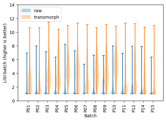
LISI-batch has greatly improved using transmorph, meaning batches are now way better mixed.

# LISI-class (lower is better)
labels = []
plt.figure(figsize=(6,4))
add_label(plt.violinplot(lisi_class_bef, positions=positions - .15), "raw")
add_label(plt.violinplot(lisi_class_aft, positions=positions + .15), "transmorph")
plt.ylim(0, 8)
plt.xticks(positions, chen_10x.keys(), rotation=90)
plt.xlabel("Batch")
plt.ylabel("LISI-class (lower is better)")

plt.legend(*zip(*labels), loc=2)
pass

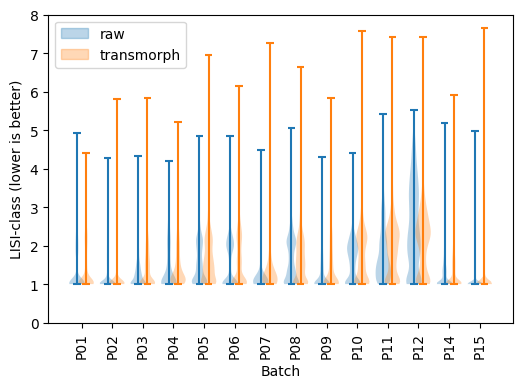
LISI-class has also consistently decreased using transmorph except for P10 and P11, meaning cell types are better separated.

References

[1] Chen, Y. P., Yin, J. H., Li, W. F., Li, H. J., Chen, D. P., Zhang, C. J., … & Ma, J. (2020). Single-cell transcriptomics reveals regulators underlying immune cell diversity and immune subtypes associated with prognosis in nasopharyngeal carcinoma. Cell research, 30(11), 1024-1042.

[2] Haghverdi, Laleh, et al. Batch effects in single-cell RNA-sequencing data are corrected by matching mutual nearest neighbors. Nature biotechnology 36.5 (2018): 421-427.

[3] Becht, Etienne, et al. Dimensionality reduction for visualizing single-cell data using UMAP. Nature biotechnology 37.1 (2019): 38-44.

[4] Korsunsky, Ilya, et al. Fast, sensitive and accurate integration of single-cell data with Harmony. Nature methods 16.12 (2019): 1289-1296.